Reductions and Completeness

Polynomial many-one reductions and the logic of hardness and completeness proofs.

Goals

• Construct polynomial many-one reductions with the correct direction, totality, and encoding analysis.
• Use transitivity and downward closure to transfer algorithms and class membership.
• Distinguish NP-hardness from NP-completeness and derive the $\mathrm P=\mathrm{NP}$ consequence correctly.
• Understand Cook–Levin as an explicit polynomial-size tableau construction.
• Prove both directions of the standard reduction $\mathrm{3SAT}\le_m^p\mathrm{IS}$.

1. A reduction is an instance compiler

For languages $A,B\subseteq\{0,1\}^*$,

means that a total, polynomial-time computable function $f$ satisfies

for every string $x$. The same output instance must preserve both yes and no answers; this is why the biconditional is indispensable.

Suppose a polynomial algorithm $D_B$ decides $B$. Then $D_A(x)=D_B(f(x))$ decides $A$. The arrow therefore points from the problem whose difficulty we already understand to the problem whose hardness we want to establish:

Reducing $B$ to $A$ only shows that access to an $A$ solver helps with $B$; it gives no evidence that $B$ is hard.

Totality and malformed inputs

The definition quantifies over strings, not only well-formed formulas or graphs. A clean construction first tests whether $x$ encodes a legal source instance. On malformed input it emits one fixed legal no-instance of $B$. This convention must agree with the source language’s malformed-input convention.

A polynomial-time transducer can print only polynomially many symbols, so its output length is polynomially bounded. Nevertheless, a proof should state the bound explicitly, especially when numbers are binary encoded.

2. Transitivity, closure, and algorithm transfer

Transitivity. If $A\le_m^p B$ via $f$ and $B\le_m^p C$ via $g$, then $A\le_m^p C$ via $h=g\circ f$.

Correctness.

Complexity. Suppose $f$ runs in time $p(n)$ and $g$ in time $q(m)$. Then $|f(x)|\le p(|x|)$ up to a harmless constant, because writing output costs time. Hence

a polynomial. Saying merely “a composition of polynomial algorithms is polynomial” hides this essential output-length bridge.

Downward closure. If $A\le_m^p B$ and $B\in\mathrm P$, then $A\in\mathrm P$. The same statement holds with NP or coNP in place of P.

For NP, let $V_B(y,w)$ verify $B$. Verify $A$ by computing $f(x)$ and running $V_B(f(x),w)$. The certificate bound remains polynomial because $|f(x)|$ is polynomial in $|x|$. For coNP, apply the same argument to complements: the biconditional gives

This closure fact explains why a single reduction can move an upper bound backward along its arrow.

3. Hardness, completeness, and the P=NP consequence

A language $B$ is NP-hard if

It is NP-complete if additionally $B\in\mathrm{NP}$. The membership proof is usually a verifier; the hardness proof usually starts from an already NP-complete problem. An NP-hard language need not even be decidable, so hardness alone never establishes completeness.

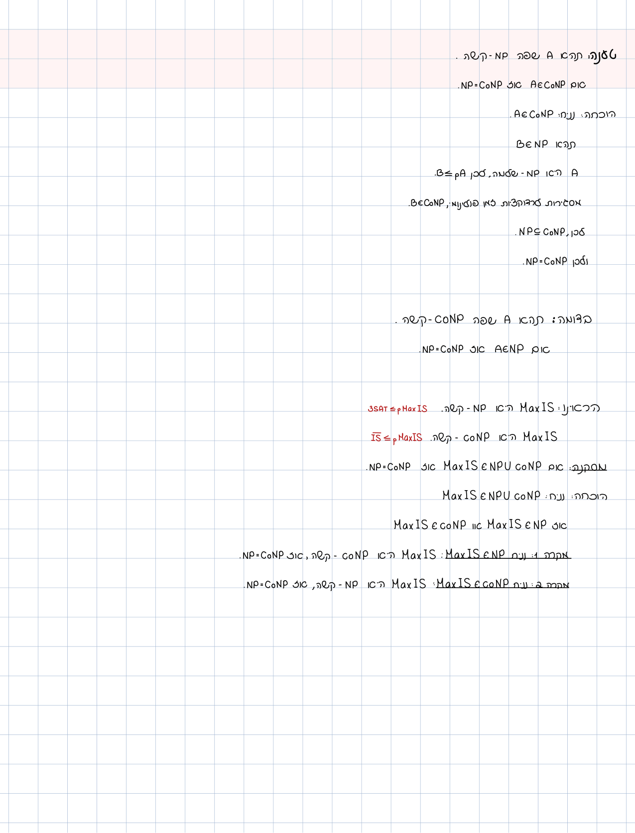
Theorem. If an NP-complete language $B$ belongs to P, then $\mathrm P=\mathrm{NP}$.

Proof. Let $A\in\mathrm{NP}$. Hardness gives $A\le_m^p B$. Since $B\in\mathrm P$, downward closure gives $A\in\mathrm P$. Therefore $\mathrm{NP}\subseteq\mathrm P$. The reverse containment is standard, so equality follows. $\square$

The contrapositive is also useful but conditional: if $\mathrm P\ne\mathrm{NP}$, then no NP-complete language is in P. We do not currently know the premise.

4. Cook–Levin: computation becomes a formula

Cook–Levin proves SAT NP-complete. SAT is in NP because an assignment can be evaluated in polynomial time. Hardness is the deeper part: for every $L\in\mathrm{NP}$ and input $x$, construct a Boolean formula $\Phi_{N,x}$ satisfiable exactly when an NTM $N$ has an accepting computation on $x$.

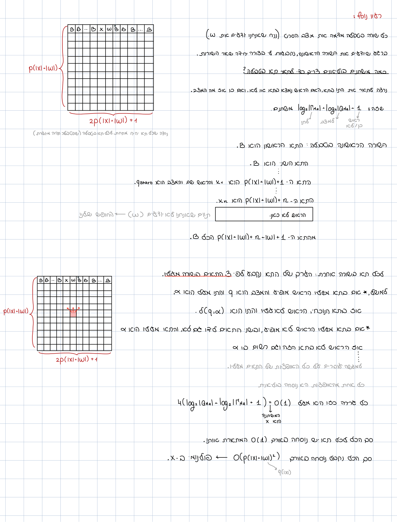
Assume every branch of $N(x)$ halts within $T=p(|x|)$ steps. During that time the head can visit only $O(T)$ tape cells. Pad shorter accepting runs with a self-looping accept state, so every relevant history has exactly $T$ rows. A tableau is a $T\times S$ grid, $S=O(T)$, whose row $t$ is the complete configuration at time $t$.

Tableau variables

Let the finite alphabet

contain ordinary tape symbols and marked symbols $(q,a)$ meaning “the head is here, the state is $q$, and the scanned symbol is $a$.” Introduce

for $0\le t<T$, $0\le i<S$, and $s\in\Gamma'$. Its intended meaning is that cell $i$ of row $t$ contains symbol $s$.

There are $O(TS|\Gamma'|)=O(T^2)$ variables because $N$ is fixed and $|\Gamma'|$ is constant.

Uniqueness constraints

Every tableau location contains exactly one symbol:

enforces at least one, while for every $s\ne r$,

enforces at most one. Across $TS$ cells this contributes $O(T^2)$ clauses for a fixed machine alphabet. Exactly one marked state/head symbol per row can be imposed similarly, or derived from a carefully chosen local-rule system plus the valid start row.

Start constraints

Unit clauses fix row $0$ to the initial configuration: state $q_0$ scans the first input symbol, the remaining input symbols occupy their cells, and all unused cells contain blanks. Because $x$ is known while constructing the formula, these are literal constants encoded by unit clauses.

Acceptance constraints

Require an accepting marked symbol somewhere:

With the padded accepting self-loop, one may instead require $q_{\mathrm{acc}}$ in the final row. Either convention works, but the transition constraints and boundary treatment must match it.

Local transition constraints

A Turing transition changes only the scanned cell, the state marker, and possibly a neighboring cell receiving the head. Therefore whether a small window in row $t+1$ legally follows row $t$ depends on a constant-size window—commonly a $2\times3$ or $2\times4$ neighborhood.

For each position and each forbidden local pattern $\pi$, add a clause forbidding all its literals simultaneously:

The window size and alphabet are constants, so there are only constantly many pattern types per $(t,i)$. Boundary cells use endmarkers or separate fixed rules. These clauses enforce that unchanged distant cells stay unchanged and that the head/state update follows one legal nondeterministic transition.

Correctness: the two directions

If $N$ accepts $x$, choose an accepting branch, write its configurations as a padded tableau, and assign each $X_{t,i,s}$ according to the grid. Every uniqueness, start, acceptance, and local-transition clause is then true.

Conversely, if $\Phi_{N,x}$ is satisfiable, uniqueness decodes one symbol per location. Start clauses make row $0$ the real initial configuration. Local clauses ensure each next row is a legal successor, not merely a visually plausible row. Acceptance clauses ensure the decoded branch accepts. Therefore

Polynomial size and construction time

There are $O(T^2)$ cells. Each receives constantly many uniqueness clauses; each space-time position receives constantly many local clauses; start and accept portions are at most polynomial. Thus $|\Phi_{N,x}|=O(T^2)$ under the fixed-machine encoding, or another fixed polynomial under alternative encodings. Enumerating the clauses takes polynomial time. This size argument is what turns the tableau idea into a reduction rather than a handwave.

The usual final step converts a general formula to CNF and then to 3CNF with auxiliary variables while preserving satisfiability and polynomial size.

What a local window actually checks

Suppose the upper row contains

and $\delta(q,a)$ permits the move “write $d$, move right, enter state $q'$.” The corresponding lower-row neighborhood must be

For a left move, the state marker moves onto the left symbol instead. If the head lies outside a window, the lower middle symbol must equal the upper middle symbol. The finite list of allowed windows contains these cases for every transition in $\delta$, together with ordinary copy windows.

To encode “this window is one of the allowed ones” in CNF, it is convenient to enumerate every forbidden assignment to its constant number of positions. If a forbidden assignment sets literals $L_1,\ldots,L_r$ true, the clause

excludes precisely that assignment. Here $r$ is a machine-dependent constant. Overlapping windows are crucial: agreement on their shared cells stitches local legality into one globally legal successor configuration. Without overlap, unrelated legal fragments could be combined into an impossible row.

For explicit accounting, write $g=|\Gamma'|$. Location constraints use $TS$ clauses of width $g$ for “at least one” and $TS\binom g2$ binary clauses for “at most one.” Start constraints use $S$ unit clauses. A final-row acceptance condition has width at most $S|\Gamma|$. If $F$ is the constant number of forbidden window patterns, transitions use at most $F(T-1)(S-2)$ constant-width clauses. Since $g,F$ depend on $N$, not on $x$, the total symbol count is $O(TS)=O(T^2)$, apart from the acceptance clause’s still-polynomial width. Converting a width-$r$ clause to 3CNF introduces only $O(r)$ variables and clauses, so polynomial size survives.

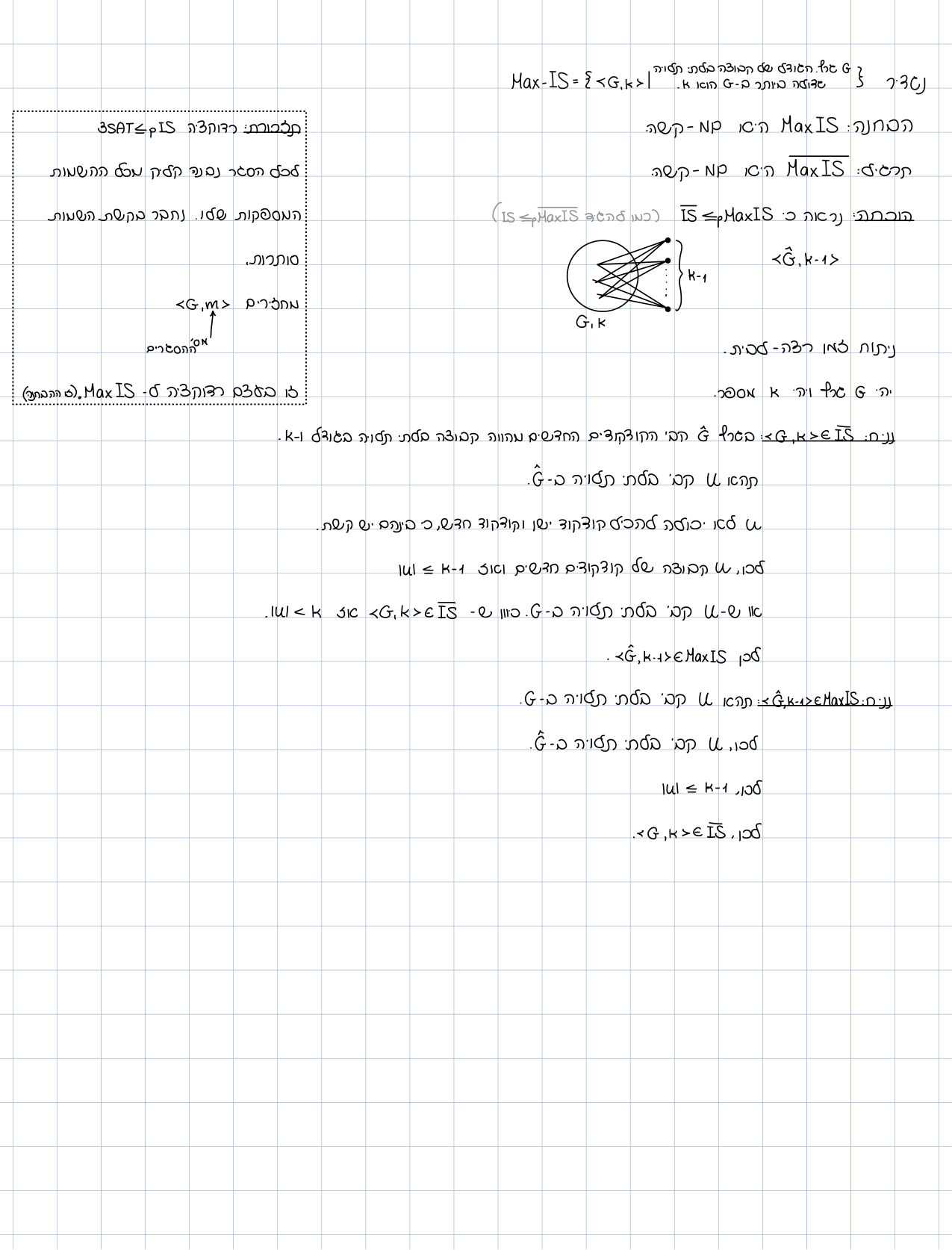
5. Full reduction: 3SAT to Independent Set

Let

be a 3CNF formula, allowing repeated literals if the chosen 3SAT definition does. Build a graph $G_\varphi$:

1. Create one vertex $v_{i,j}$ for each literal occurrence $\ell_{i,j}$ in clause $C_i$.
2. Connect every pair of vertices belonging to the same clause. Each clause gadget is a triangle (or a clique for clauses represented with fewer distinct occurrences).
3. Connect two vertices from different clauses whenever their literals are complementary, $x$ and $\neg x$.
4. Output $(G_\varphi,k=m)$.

The graph has $3m$ vertices and at most $3m+9\binom m2=O(m^2)$ edges, so it is polynomial to construct.

Forward direction

Assume $\varphi$ is satisfiable under assignment $\alpha$. In each clause choose one occurrence made true by $\alpha$, and put its vertex in $S$. Exactly one is chosen from each clause, hence $|S|=m$. No two chosen vertices lie in one clause, so no clause edge joins them. Nor can two chosen literals be complementary: one assignment cannot make both $x$ and $\neg x$ true. Therefore $S$ is independent.

Reverse direction

Assume $G_\varphi$ has an independent set $S$ of size $m$. Since every clause gadget is a clique, $S$ contains at most one vertex from each clause. There are exactly $m$ clauses and $m$ selected vertices, so it contains exactly one from every clause.

No selected pair is connected by a conflict edge, so the selected literals contain no complementary pair. Define a partial assignment making each selected literal true. It is consistent: no variable is forced both ways. Extend arbitrarily to unmentioned variables. Each clause contains its selected true literal, so every clause—and therefore $\varphi$—is satisfied.

Thus

IS is in NP: list $k$ distinct vertices and test every pair for nonadjacency. Since 3SAT is NP-hard, this proves IS NP-complete.

Mini-example

For

create three triangles, one per clause, and set $k=3$. Add conflict edges between the first occurrence of $x$ and the second occurrence of $\neg x$; between every $y$ occurrence and the third clause’s $\neg y$; and any other complementary pair that appears. Repeated positive occurrences such as $z$ are not conflicts with one another.

The assignment $x=1,y=1,z=1,w=0$ satisfies the formula. One resulting independent set chooses $x$ from $C_1$, $y$ from $C_2$, and $z$ from $C_3$. These vertices lie in different triangles and no selected literals are complementary.

Now start from an arbitrary independent set of size three. It cannot choose two vertices from one triangle. Because there are three triangles, it chooses one per clause. It cannot, for example, choose $y$ from $C_1$ and $\neg y$ from $C_3$, because those vertices have a conflict edge. Thus its three chosen literals form a consistent partial assignment and certify all three clauses simultaneously.

This example also shows why selecting merely two nonconflicting vertices would not suffice: two clauses could be represented while the third remained unsatisfied. The threshold is part of the reduction’s logic, not a cosmetic parameter.

6. A reduction-proof checklist

Before declaring a reduction complete, verify five separate obligations:

1. Input and output. State the exact decision-language encodings and parameters.
2. Construction. Describe $f(x)$ on legal and malformed source strings.
3. Forward implication. Transform every source witness into a target witness.
4. Reverse implication. Decode every target solution meeting the threshold into a source solution.
5. Resources. Bound output objects, bit lengths, and construction time in the encoded source length.

For 3SAT→IS, these become: $3m$ occurrence vertices; clause and conflict edges; one true occurrence per clause in the forward direction; one consistent occurrence per clause in the reverse direction; and $O(m^2)$ output size. Keeping the obligations separate prevents a persuasive gadget drawing from replacing the formal proof.

7. Direction tested with a hypothetical solver

A reliable direction test is to write the algorithm that would follow from the reduction. Suppose the goal is to show a new problem $B$ is hard and SAT is the known-hard source. Given a SAT formula $\varphi$, compute $f(\varphi)$, call a hypothetical solver for $B$ once, and return that answer. This algorithm exists precisely when

Thus the required statement is $\mathrm{SAT}\le_m^pB$. If the construction instead starts from a $B$ instance and calls a SAT solver, it proves $B\le_m^p\mathrm{SAT}$—an upper-bound style result that every NP language already has after Cook–Levin.

Reductions also compose into a network. From

transitivity gives $\mathrm{SAT}\le_m^p\mathrm{IS}$. There is no need to rebuild the Cook–Levin tableau inside the graph reduction. This modularity is the practical value of completeness: after one universal source is established, later proofs can begin from whichever complete problem best matches the target structure.

Finally, a reduction does not compare the running times of the best algorithms in both directions. From $A\le_m^pB$, a fast $B$ algorithm gives a fast $A$ algorithm up to polynomial overhead. A fast $A$ algorithm says nothing about $B$, and the reduction alone does not prove that $B$ is strictly harder.

Common mistakes

1. Reversing the hardness arrow.
2. Proving only “yes maps to yes” rather than an iff.
3. Ignoring malformed strings or claiming a partial mapping.
4. Measuring numeric runtime in value rather than binary length.
5. Declaring NP-completeness after hardness without proving membership.
6. Saying “Cook–Levin records a computation” without variables, constraints, correctness, and size.
7. In 3SAT→IS, forgetting clause edges or complementary-literal edges.
8. In the reverse proof, failing to explain why size $m$ forces one choice per clause.

Exercises

Exercise 1 — Direction of hardness

Let $A\le_p B$. Prove: if $B\in\mathrm P$ then $A\in\mathrm P$. Explain what flows backward and what flows forward along the reduction arrow.

Exercise 2 — Two obligations for completeness

Define NP-completeness. Prove why NP membership alone or hardness alone is insufficient.

Exercise 3 — Local windows in Cook–Levin

Explain why local-window constraints on the computation tableau suffice to enforce a legal TM computation.

Exercise 4 — $k=m$ in 3SAT→IS

In the standard reduction from 3SAT to Independent Set with parameter $k=m$ (number of clauses), prove why choosing $k<m$ breaks equivalence.

Exercise 5 — Transitivity and output size

Prove $\le_p$ is transitive, emphasizing why $|f(x)|$ must be polynomial.

Summary

A reduction is an instance compiler with a direction. Completeness needs membership and hardness; direction and size mistakes are classic exam traps.

Guided practice

Task 1 — Refute a wrong direction

A student “proves” $B$ is hard via a reduction $B\le_p A$ where $A$ is easy. What is wrong?

Task 2 — Partial reduction writeup

In a graph reduction only “if the formula is satisfiable then an independent set exists” is proved. Which parts are missing?

Task 3 — From Cook–Levin to 3SAT-completeness

Outline how one passes from SAT to 3SAT while preserving NP-completeness (gadget idea, not a full proof).

Sources

Course evidence

• Current Semester A transcript 9: polynomial many-one reductions, direction, transitivity, and closure.
• Current Semester A transcript 10: NP-hardness, NP-completeness, and the consequences of a polynomial algorithm for a complete problem.
• Current Semester A transcripts 12–13: the Cook–Levin computation tableau, local consistency, acceptance, and polynomial-size accounting.
• Current Semester A transcript 14: SAT/3SAT graph gadgets, including the independent-set construction.
• Merged course summary, pp. 43–49: polynomial reductions and completeness; pp. 50–54: Cook–Levin only; pp. 55–57, 64–66, and 72–75: the graph-problem family and graph reductions. No broader topic coverage is attributed to these ranges.

Textbook verification

• Sipser, Introduction to the Theory of Computation, 3rd ed., §§7.4–7.5, pp. 300–325: polynomial reducibility, Cook–Levin, and 3SAT.
• Arora–Barak, Computational Complexity: A Modern Approach (draft), §2.3, pp. 45–58: universality of tableau/Cook–Levin encodings and NP-completeness.
• Papadimitriou, Computational Complexity, Chs. 8–9: reductions, NP-completeness, and the tableau proof. Textbooks verify the standard theorem; notation and teaching order here follow the course.