Randomized Computation

Monte Carlo and Las Vegas algorithms, amplification, and Karger's random contraction method.

Goals

• Model randomized Turing machines as deterministic machines with a random tape.
• Distinguish Monte Carlo, Las Vegas, one-sided, two-sided, and zero error.
• Analyze Freivalds' test, amplification, and Karger's contraction.
• Place $\mathrm{RP}$, $\mathrm{coRP}$, $\mathrm{BPP}$, and $\mathrm{ZPP}$ correctly.

1. Random bits are not nondeterministic guesses

A probabilistic Turing machine (PTM) has ordinary work tapes plus independent fair random bits. Equivalently, at each random state it chooses one of two transitions with probability $1/2$. Fixing a random string $r$ makes the computation deterministic. If $m(|x|)$ bits are used, then

Nondeterminism asks whether some accepting branch exists. Randomization measures the fraction of accepting random strings. One rare accepting branch certifies NP acceptance but does not satisfy a bounded-error randomized definition.

Always specify the sample space, whether repetitions use fresh independent bits, and whether the guarantee is per input. The complexity classes below require their probability bound for every input, not merely on average over an input distribution.

2. Monte Carlo and Las Vegas

A Monte Carlo algorithm has a fixed runtime bound but may return a wrong answer with bounded probability. Error is one-sided when one kind of answer is always correct and two-sided when either kind can be wrong.

A Las Vegas algorithm never returns a wrong answer; its runtime is random, generally bounded in expectation. If a verifiable trial finds a correct witness with probability at least $1/4$, repeating until success is always correct and takes at most four trials in expectation. Truncating after $t$ trials yields a Monte Carlo algorithm whose timeout probability is at most $(3/4)^t$.

“Correct in expectation” is not Las Vegas. The defining property is always correct, random time.

3. Freivalds' matrix-product test

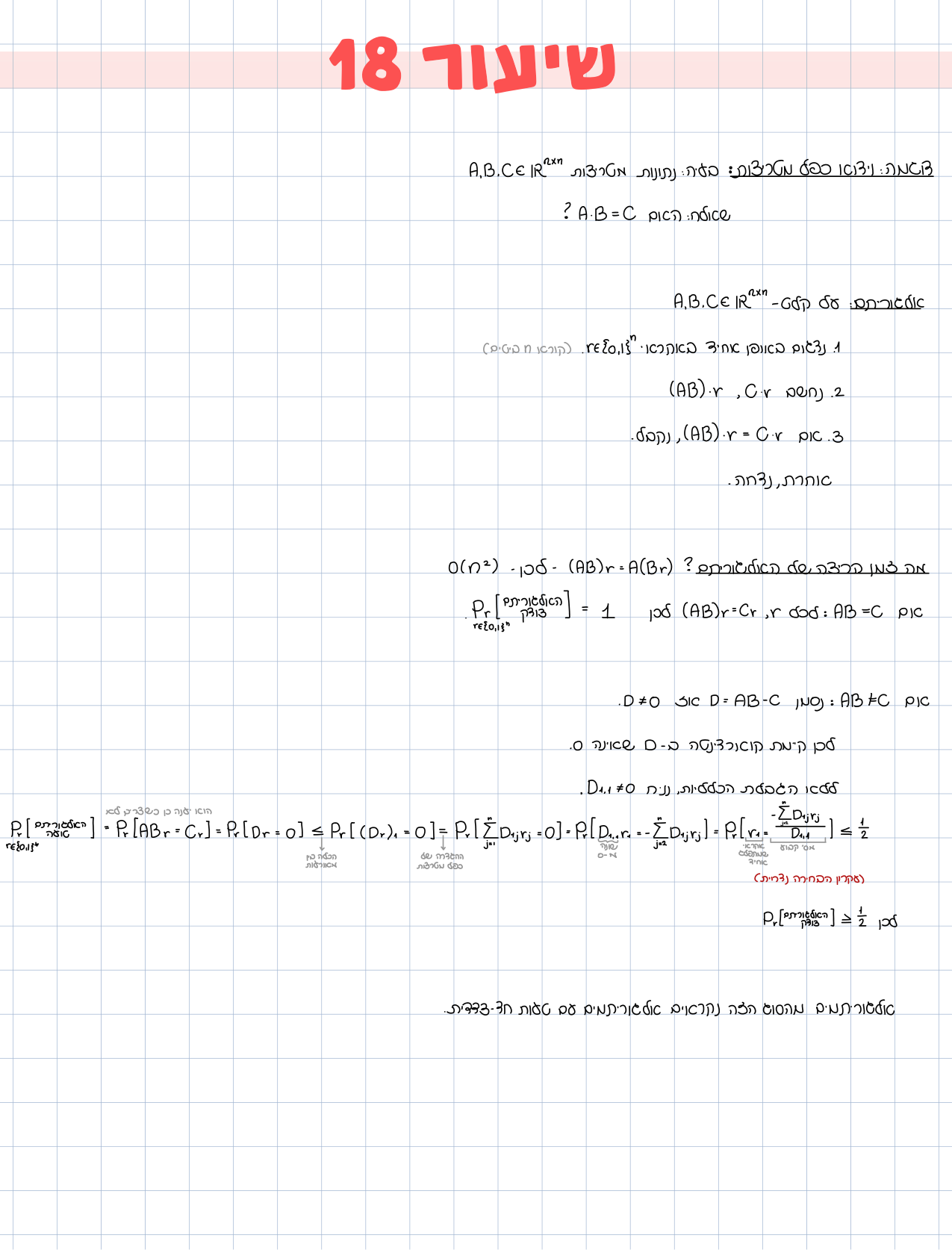
Given $n\times n$ matrices $A,B,C$ over a field, Freivalds tests $AB=C$ in $O(n^2)$ field operations:

1. Choose $r\in\{0,1\}^n$ uniformly with independent coordinates.
2. Compute $u=Br$, $v=Au$, and $w=Cr$.
3. Accept iff $v=w$.

If $AB=C$, every run accepts. If $D=AB-C\ne0$, choose a nonzero row and a coordinate $j$ with nonzero coefficient. Condition on all coordinates except $r_j$. Of its two values, at most one makes that row's dot product zero, because the two sums differ by the nonzero coefficient $D_{ij}$. Hence

The test has one-sided false-accept error. For a tight example over $\mathbb F_2$, let

$Dr=0$ exactly for $r=00$ and $r=11$, probability $1/2$. With $k$ fresh vectors, a false equality survives with probability at most $2^{-k}$.

4. Amplification

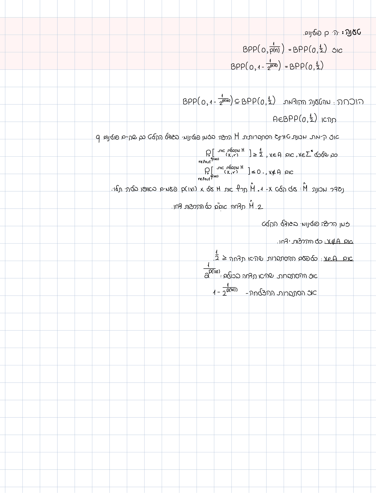
If each independent run fails with probability at most $q<1$ and any success suffices, all $k$ runs fail with probability at most $q^k$. To make this at most $\delta$, take

For one-sided error, combine runs with OR or AND in the direction preserving the perfect side. For BPP's two-sided error, take the majority of an odd number of independent runs. From success probability at least $2/3$, a Chernoff bound gives error $\exp(-\Omega(k))$, so $k=O(\log(1/\delta))$.

Amplification reduces but does not literally remove error. Reusing one random string is not independent repetition. Constants such as $1/2$ and $2/3$ are conventional because any fixed gap from $1/2$ can be amplified.

5. Randomized complexity classes

For a polynomial-time PTM $M$:

$\mathrm{ZPP}$ consists of zero-error expected-polynomial-time languages. Standard relationships are

For the equality, alternate an RP machine and a coRP machine until the first accepts or the second rejects. Neither stopping answer can be wrong, and each round has constant stopping probability. Conversely, truncate a zero-error expected-polynomial algorithm after a suitable multiple of its expectation. Markov's inequality bounds timeout; assigning timeout oppositely gives RP and coRP machines.

Whether $\mathrm{BPP}=\mathrm P$ is unknown; do not present it as a theorem.

6. Karger's random contraction

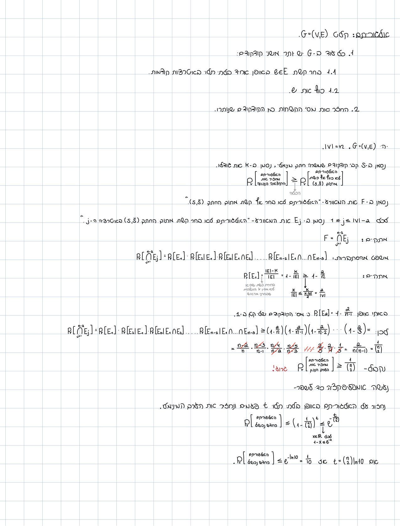
Repeatedly choose a uniformly random current edge of an undirected multigraph, contract its endpoints, delete self-loops, and retain parallel edges. At two supervertices, output their separating edges.

Fix a minimum cut $F$ of size $\lambda$. If it has survived while $i$ supervertices remain, every supervertex has degree at least $\lambda$; otherwise its incident cut is smaller. Thus there are at least $i\lambda/2$ edges, and only $\lambda$ are dangerous. The chance of contracting $F$ is at most $2/i$, so its survival probability is at least

Worked example

The telescoping product equals $2/(n(n-1))$: inverse-polynomial, not constant, success. With $R$ independent runs, failure is at most

Thus $R=\Theta(n^2\log(1/\delta))$ gives failure at most $\delta$. For $n=4$, the fixed-cut bound is $1/6$. A cycle $C_4$ has several minimum cuts, so finding some optimum can be likelier. Parallel edges remain because multiplicity is both cut capacity and sampling weight.

7. Compare the guarantees

• Freivalds: bounded $O(n^2)$ time and one-sided error; repeated error at most $2^{-k}$.
• BPP: polynomial worst-case time and two-sided error bounded away from $1/2$ on every input.
• Las Vegas/ZPP: no wrong answer and expected polynomial time.
• Karger: every output is feasible, but one run is optimal only with inverse-polynomial probability.

For Karger, “failure” means suboptimal, not malformed. Feasibility and quality are separate claims.

Common mistakes

• Treating random and nondeterministic branches identically.
• Defining correctness only on average over inputs.
• Claiming independence when runs reuse randomness.
• Combining one-sided repetitions in the wrong direction.
• Calling expected correctness “Las Vegas.”
• Dropping parallel edges during contraction.
• Saying amplification makes error exactly zero.

Visualizations

Also draw a PTM tree with equally weighted leaves. Label NP “at least one accepting leaf,” RP “none on no-instances and many on yes-instances,” and BPP “a strong majority agrees.”

Exercises

Exercise 1 — Freivalds when $AB=C$

What happens in Freivalds' algorithm when $AB=C$? Prove there is no false rejection in that case.

Exercise 2 — Amplification to $2^{-40}$

An $\mathrm{RP}$-style algorithm (on yes-instances $\Pr[\text{accept}]\ge1/2$; on no-instances no false accepts) is run $k$ independent times. Accept if at least one run accepts. How many repetitions reduce the false-reject probability on a yes-instance to $\le2^{-40}$?

Exercise 3 — One accepting path is not RP

Prove that a single accepting path of a PTM does not establish membership in $\mathrm{RP}$.

Exercise 4 — $\mathrm{ZPP}=\mathrm{RP}\cap\mathrm{coRP}$

Explain both directions of $\mathrm{ZPP}=\mathrm{RP}\cap\mathrm{coRP}$.

Exercise 5 — Karger's edge lower bound

Why does Karger's proof lower-bound the current number of edges by $i\lambda/2$ when $i$ supernodes remain and the min-cut is $\lambda$?

8. Detailed probability walkthroughs

Turning biased random choices into fair-bit computation

The PTM definition uses fair bits for convenience, not because algorithms may only sample powers of two. To sample uniformly from $\{1,\ldots,6\}$, read three bits as an integer in $\{0,\ldots,7\}$; reject $6,7$ and retry. Every accepted value has the same probability, and acceptance occurs with probability $3/4$, so the expected number of rounds is $4/3$. This is a small Las Vegas sampler. A hard worst-case cutoff would introduce a failure event and make it Monte Carlo.

If an algorithm says “choose a random edge,” it means uniform among current edge copies. Sampling endpoints uniformly would be a different distribution and would invalidate Karger's calculation. Translating prose into a precise random-bit procedure is part of specifying the algorithm.

Freivalds with integers and fields

Over the integers, the same binary-vector argument works because a nonzero coefficient cannot disappear when $r_j$ flips. Implementations must account for arithmetic cost and overflow. One can instead compute modulo a suitably chosen prime, but then a nonzero integer error matrix might become zero modulo that prime. If the prime is fixed, this is a new source of error; if it is selected from a suitable range, its probability must be analyzed separately. The clean theorem stated above assumes exact field operations and $AB\ne C$ in that field.

Freivalds verifies a claimed product; it does not compute the product. This distinction explains the speedup. Computing $Br$, then $A(Br)$, uses two matrix-vector products, while explicitly forming $AB$ would compute all pairwise row-column products.

Exact amplification arithmetic

Suppose a Freivalds run costs $2n^2+O(n)$ operations and a false product passes with probability at most $1/2$. Ten runs cost $O(10n^2)=O(n^2)$ because ten is constant, and reduce error to $1/1024$. To reach error at most $1/n^c$, choose

The runtime becomes $O(n^2\log n)$. To reach exponentially small $2^{-n}$ error requires $n$ runs and $O(n^3)$ elementary time, erasing the asymptotic advantage over elementary multiplication. Error targets and runtime must be analyzed together.

For BPP majority, simple multiplication of failure probabilities is wrong because majority can be wrong even when some runs are correct. Let $Y_i$ indicate correctness and use concentration around $\mathbb E[\sum Y_i]\ge2k/3$. A majority error means falling below $k/2$, a linear deviation, which Chernoff bounds exponentially. Independence is again essential.

Converting expected time safely

Let a zero-error algorithm have expected runtime at most $p(n)$. Markov gives

Stop it after $2p(n)$ steps. For an RP version, accept only if the algorithm halted and answered yes; otherwise reject. No no-instance is falsely accepted, while a yes-instance is accepted with probability at least $1/2$. For coRP, accept on timeout and preserve the opposite perfect side. Constants can then be amplified.

The known expectation bound must be uniform and computable enough to set the cutoff. Merely observing good average runtime in experiments does not prove ZPP membership.

Karger: conditioning one stage at a time

The min-cut degree argument is conditional. After arbitrary safe contractions, each current supervertex represents a nonempty original vertex set. Its current incident edges form a cut of the original graph, so its degree is at least $\lambda$. This is why the same lower bound remains valid throughout a successful prefix.

At $i$ vertices, survival probability for the next contraction is at least $(i-2)/i$. Multiplying conditional probabilities is legitimate:

No claim is made that contraction events are independent. They are strongly dependent; conditioning is the correct tool. The product telescopes because numerators $n-2,n-3,\ldots,1$ cancel almost all denominator factors $n,n-1,\ldots,3$.

A small contraction trace

Take a square with one diagonal. Its minimum cut has size two at either vertex not incident to both diagonal ends. Fix such a cut and color its two edges red. If the first chosen edge is not red, contract it and keep every resulting parallel edge. Recompute the current edge multiset before the next uniform choice. If a red edge is ever selected, that fixed partition can no longer be output; if neither is selected until two supervertices remain, all red copies cross the final cut and the run has recovered it.

The algorithm need not know $\lambda$ or the protected cut. They exist only in the analysis. This is a common randomized-proof pattern: fix a desirable witness, calculate the probability that random operations preserve it, then repeat.

9. Designing a randomized proof

Use the following checklist:

1. Define the random tape or explicit random variables.
2. State exactly which outputs count as errors.
3. Prove the runtime bound separately from correctness.
4. Condition on history when choices change the future sample space.
5. Use fresh randomness before multiplying probabilities.
6. State whether the result is worst-case time, expected time, expected quality, or high-probability correctness.
7. For optimization, prove every output is feasible even on unsuccessful runs.

These distinctions prevent a frequent category error: an expected approximation ratio, a bounded-error decision algorithm, and a zero-error expected-time algorithm are three different guarantees even when all use coins.

Sanity checks on class definitions

An RP machine may reject a yes-instance, but repeated OR preserves the rule that no no-instance is ever accepted. A coRP machine may accept a no-instance, and repeated AND preserves its perfect yes-side. For BPP, neither raw OR nor raw AND is appropriate because it drives one error down while driving the other up; majority balances both.

The class bound is over the machine's coins for each fixed input. It gives no promise that one random seed works for every input of a given length. Fixing a globally good seed is a derandomization question and generally needs an additional argument. Likewise, pseudorandom generators cannot simply replace true coins unless their fooling property is proved for the computation being run.

When reporting a randomized algorithm, include the confidence parameter $\delta$ in its runtime. “With high probability” conventionally means failure at most $1/n^c$ for a desired constant $c$, which usually costs $O(\log n)$ repetitions from constant error and $O(n^2\log n)$ contractions from Karger's inverse-polynomial single-run success.

Summary

Randomness is not nondeterminism: probabilities, error sidedness, and amplification are required. RP, coRP, BPP, and ZPP encode different guarantees.

Guided practice

Task 1 — Monte Carlo versus Las Vegas

Distinguish Monte Carlo from Las Vegas in time, error, and an example (Freivalds versus rejection sampling).

Task 2 — RP versus NP

Write the quantifiers/probabilities for $\mathrm{NP}$ and $\mathrm{RP}$ on yes- and no-instances.

Task 3 — Randomized proof template

Outline a five-step template for proving a randomized algorithm (as taught in the unit).

Source trail and authority

• Student-summary evidence (scope only): סיכומי שיעור/סיכום ממוזג.pdf, pp. 86–94, 96, and 136–139 (the summary's randomized-computation treatment). Karger's contraction algorithm is absent from the merged summary, so its algorithm and analysis above are textbook-supported enrichment only. The student summary establishes course emphasis, not authority for constants or class equalities.
• Textbook authority: Arora–Barak, Computational Complexity: A Modern Approach, 2007 draft, Ch. 7, §§7.1–7.4, book pp. 115–124; Papadimitriou, Computational Complexity, Ch. 11, §§11.1–11.3, pp. 241–267; Sipser, 3rd ed., §10.2, pp. 396–408.
• Editorial status: class definitions, Freivalds' bound, amplification, and the contraction product were checked against these textbook frameworks and standard derivations. Reviewed; high confidence.