Approximation Algorithms

Approximation ratios and proof patterns for Vertex Cover, Max-Cut, metric TSP, and Bin Packing.

Goals

• Separate optimization problems from their threshold decision versions.
• State and prove approximation guarantees for minimization and maximization.
• Analyze four representative algorithms and recognize their proof patterns.
• Treat Bin Packing's additive guarantees carefully.

1. Optimization is not a decision language

A decision problem asks for one bit. For example, VC-DEC asks whether a graph has a vertex cover of size at most $k$. The associated optimization problem MIN-VC asks for the smallest cover itself (or its size). NP-completeness is formally a property of the decision language; approximation is a guarantee about the optimization objective.

Threshold queries connect the two. If objective values are integers bounded by a polynomial number of bits and we can answer “is $\mathrm{OPT}\le k$?”, binary search finds the optimal value. A standard self-reduction can often recover a witness. Conversely, an optimizer answers every threshold question. This connection does not mean that an approximation algorithm decides the exact language: a $2$-approximation returning cost $12$ cannot decide whether $\mathrm{OPT}\le7$.

Write an optimization problem as instances $I$, feasible solutions $F(I)$, and objective $\operatorname{val}(I,S)$. Let $\mathrm{OPT}(I)$ be the best feasible value. A polynomial-time algorithm must first output $S\in F(I)$; only then does the ratio matter.

Ratio conventions

For minimization, an $\alpha$-approximation, $\alpha\ge1$, satisfies

For maximization we use the same factor-above-one convention:

Some texts instead report a maximization performance fraction $\rho\in[0,1]$ with $A(I)\ge\rho\mathrm{OPT}(I)$. Thus “a $1/2$ guarantee” and “a factor-$2$ approximation” may describe the same Max-Cut result. State the convention. The guarantee is worst-case, per instance, and includes polynomial running time; good experiments alone establish only a heuristic.

2. Minimum Vertex Cover: maximal matching

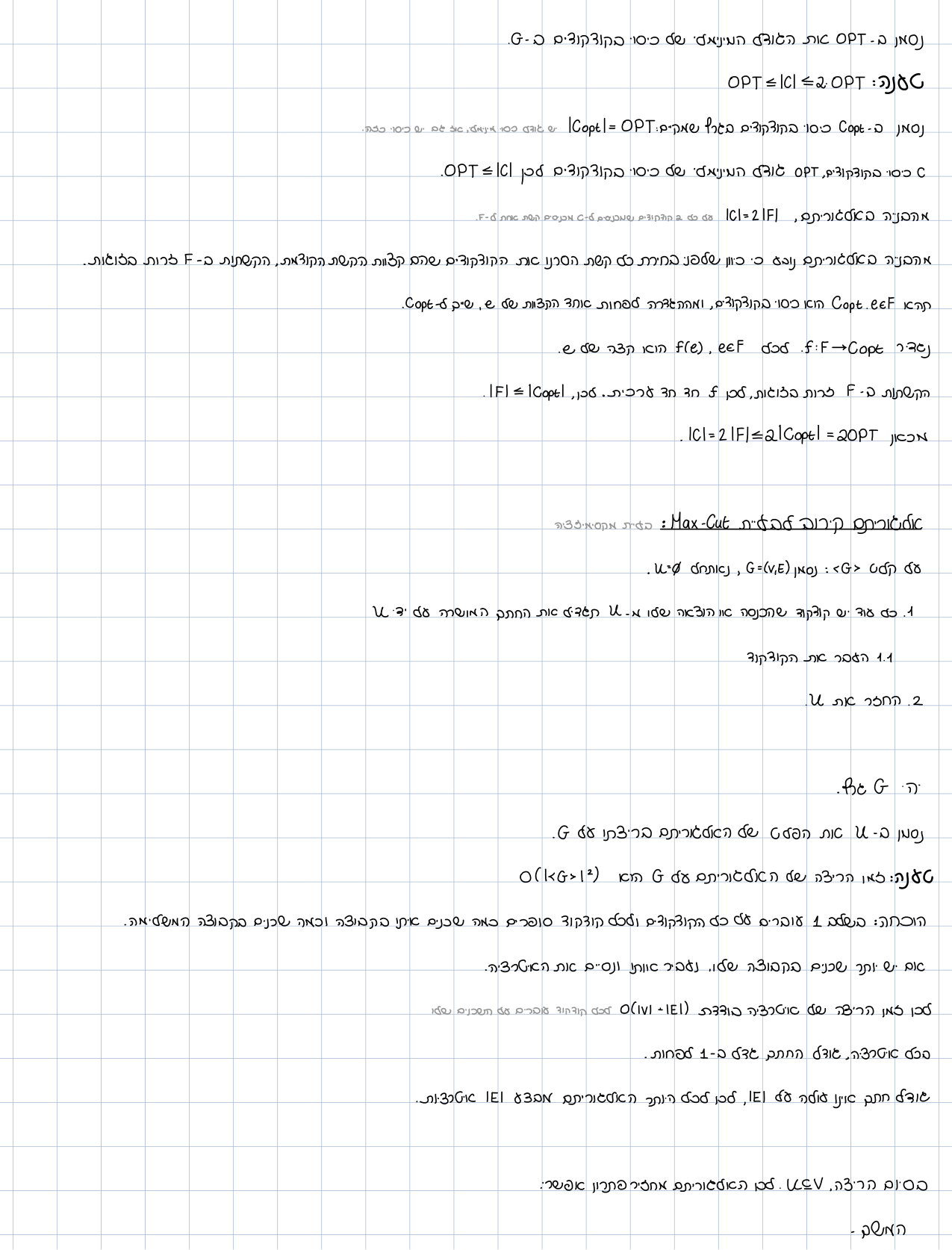
Algorithm. Start with $C=\varnothing$. While an uncovered edge $\{u,v\}$ remains, put both $u,v$ in $C$ and delete all edges incident to either endpoint. Return $C$. The chosen edges form a maximal matching $M$.

Theorem. The algorithm is a $2$-approximation for unweighted Minimum Vertex Cover.

Proof walkthrough.

1. Feasibility. When the loop stops no edge remains uncovered. Equivalently, if an edge had neither endpoint in $C$, it could have been added to $M$, contradicting maximality.
2. Lower bound. Every vertex cover must contain at least one endpoint of each edge of $M$. Matching edges are vertex-disjoint, so one selected vertex cannot cover two of them. Hence $\mathrm{OPT}\ge |M|$.
3. Charge the output. The algorithm takes exactly two endpoints per matched edge: $|C|=2|M|\le2\mathrm{OPT}$.

On the path $1-2-3-4$, choosing edges $\{1,2\}$ and $\{3,4\}$ returns all four vertices, while $\{2,3\}$ is an optimum cover of size two. The factor can therefore be tight for this algorithm. “Maximal” means no edge can be added; it does not mean maximum cardinality.

3. Max-Cut: half of all edges

For an undirected graph $G=(V,E)$, a cut $(S,V\setminus S)$ has value equal to the number (or total nonnegative weight) of crossing edges.

Randomized algorithm. Independently put every vertex on either side with probability $1/2$. For each edge $e=\{u,v\}$, let $X_e=1$ if its endpoints differ. Then $\Pr[X_e=1]=1/2$, and linearity of expectation gives

Because $\mathrm{OPT}\le |E|$, the expected cut is at least $\mathrm{OPT}/2$. No independence among the $X_e$ variables is required for this sum. Repeating and keeping the best cut improves confidence, but the expectation statement already proves existence.

There is also a deterministic form. Process vertices one at a time, choosing the side that leaves the conditional expected final cut no smaller. This method of conditional expectations returns a cut of value at least $|E|/2$. An elementary local-improvement view gives the same bound: move any vertex having more neighbors on its own side than across. Each move strictly increases the integer cut value, so the process stops; at termination every vertex has at least half its incident edges crossing. Summing crossing degrees counts every crossing edge twice, yielding $2|\delta(S)|\ge |E|$.

Example. A triangle has three edges and optimum two. Random assignment has expected $3/2$, while local improvement returns a cut of size two. The analysis promises only at least $1.5$ in expectation (hence at least two for some integral cut), not that every random run cuts half the edges.

4. Metric TSP: the double-tree algorithm

General TSP admits no useful metric shortcut argument. Here the input is a complete weighted graph whose nonnegative distances satisfy symmetry and the triangle inequality

Algorithm.

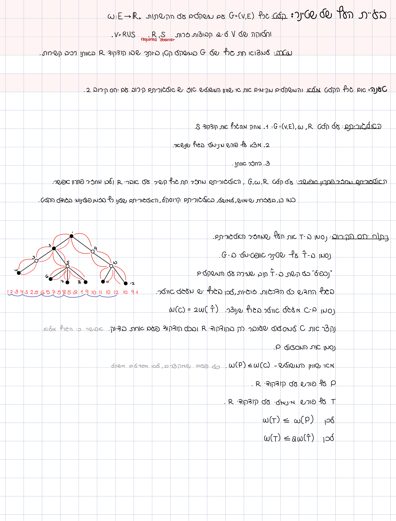
1. Compute a minimum spanning tree $T$.
2. Double every edge of $T$. All degrees are even, so the multigraph has an Euler tour.
3. Traverse an Euler tour and shortcut already visited vertices, finally returning to the start.

Theorem. Double-tree is a $2$-approximation for metric TSP.

Proof walkthrough. Delete any edge from an optimal Hamiltonian cycle; what remains is a spanning tree, so $w(T)\le\mathrm{OPT}$. Doubling gives an Eulerian multigraph of weight $2w(T)$. Whenever the Euler walk would revisit vertices, replace a subpath by the direct edge. Triangle inequality says shortcutting cannot increase cost. The resulting Hamiltonian tour therefore costs at most

Worked example. Put four points at the corners of a unit square with Euclidean distances. An MST uses three unit sides, so its doubled weight is $6$. One Euler traversal may revisit a corner; shortcutting can produce the perimeter tour of cost $4$, which is optimal. The guarantee remains $2$, even though this instance performs better.

The most common invalid proof applies shortcutting without a metric. If a missing diagonal is represented by a very expensive direct edge, replacing a two-edge detour can increase cost.

5. Bin Packing: asymptotic and additive care

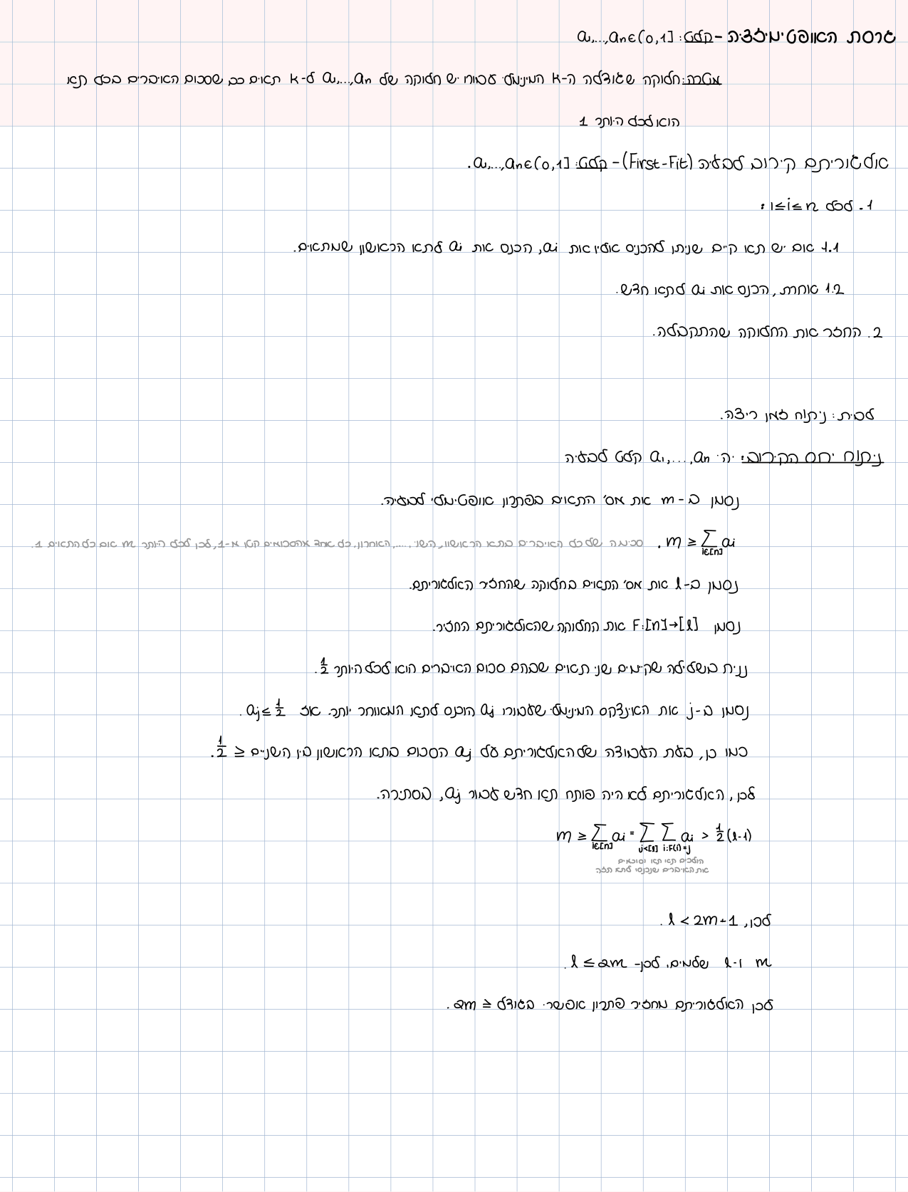
Items have sizes $s_i\in(0,1]$ and bins have capacity $1$. The goal is to minimize the number of bins. The volume lower bound is

but volume alone can be weak because items cannot be split.

Next Fit (NF). Keep one open bin. Place the next item if it fits; otherwise close that bin and open a new one. If NF uses $m$ bins, every consecutive pair of bins has total load greater than $1$: the first item of the later bin did not fit in the earlier one. Pairing bins gives

so $m\le2\,\mathrm{OPT}$ (a sharper statement is $m<2\mathrm{OPT}+1$). The algorithm is online: it sees no future items.

First Fit Decreasing (FFD). Sort items in nonincreasing order, then put each into the first bin with enough room. FFD is substantially stronger. A classical theorem gives

This is an absolute bound with an additive constant, and implies asymptotic ratio $11/9$. Do not erase the additive term when $\mathrm{OPT}$ is small. The full FFD proof uses a detailed classification of item sizes and is beyond this lesson; the course-summary pages motivate the algorithm, while textbook authority is used here only for the general approximation framework.

Example. For items $0.6,0.6,0.4,0.4$, NF in that order makes two perfect bins. In the order $0.6,0.4,0.6,0.4$ it also makes two; but order sensitivity appears immediately in larger examples, which is why decreasing-order preprocessing matters.

6. A reusable proof template

For every claimed approximation:

1. Specify the input assumptions and objective.
2. Give executable polynomial-time pseudocode.
3. Prove the output is feasible.
4. Find a lower bound on $\mathrm{OPT}$ for minimization, or an upper bound for maximization.
5. Relate the algorithm's value to that bound.
6. State whether the result is deterministic, expected, high-probability, absolute, or asymptotic.

Matching size lower-bounds Vertex Cover; total edge weight upper-bounds Max-Cut; MST weight lower-bounds metric TSP; total item volume lower-bounds Bin Packing. These simple certificates are the engines of the analyses.

Common mistakes

• Calling an optimization problem “NP-complete” without identifying its decision version.
• Proving a bound on cost but not feasibility or polynomial runtime.
• Inverting minimization and maximization inequalities.
• Treating expected performance as a guarantee for every random run.
• Shortcutting a TSP walk without triangle inequality.
• Reporting an asymptotic Bin Packing ratio as an exact bound for every instance.

Visualizations

For a board visualization, draw four “proof bridges”: matched edges $\to$ VC lower bound; all edges $\to$ Max-Cut upper bound; optimal tour minus one edge $\to$ MST; total item volume $\to$ bins. Label each bridge with the direction of its inequality.

Exercises

Exercise 1 — Factor from a bound

A minimization algorithm returned $30$, and you proved $\mathrm{OPT}\ge20$. Which approximation factor did you prove? Why need you not know exact $\mathrm{OPT}$?

Exercise 2 — Vertex Cover via maximal matching

Prove that taking both endpoints of a maximal matching is a $2$-approximation. Distinguish maximal from maximum matching.

Exercise 3 — Max-Cut expectation

Prove $\mathbb E[X]\ge\tfrac12\sum_e w_e$ for a fair random cut with nonnegative weights, even with dependence. When do negative weights break the argument?

Exercise 4 — Metric TSP

Outline the double-tree $2$-approximation under triangle inequality. What fails without it?

Exercise 5 — Bin packing volume

NF used $9$ bins. What does the adjacent-bin pairing argument say about $\mathrm{OPT}$? Why does an asymptotic $11/9$ ratio not replace additive constants on small instances?

Summary

Approximation is a worst-case theorem: a feasible polynomial-time solution versus a bound on $\mathrm{OPT}$. Bound direction and problem hypotheses are part of the proof.

Guided practice

Task 1 — Bound direction

A VC run selected $6$ matching edges ($12$ vertices). You also found a hand cover of size $8$. What does each number prove about the factor?

Task 2 — Expectation versus derandomization

Random Max-Cut may return an empty cut on one run. How do conditional expectations turn an expectation guarantee into a deterministic algorithm?

Task 3 — Approximation versus NP-completeness

Why does a polynomial approximation algorithm for an optimization problem not contradict NP-completeness of the decision version?

Source trail and authority

• Student-summary evidence (scope only): סיכומי שיעור/סיכום ממוזג.pdf, pp. 58–63, 67, and 76–80. Pages 79–80 discuss Steiner Tree and use a related MST/doubling/shortcut pattern; they do not explicitly present metric TSP. Accordingly, the metric-TSP lesson above is supported by the textbooks, not attributed to the merged summary. The summary is student-authored evidence of course emphasis, not final authority.
• Textbook authority: Sipser, Introduction to the Theory of Computation, 3rd ed., §10.1, pp. 393–396 (approximation framework); Papadimitriou, Computational Complexity, Ch. 13, especially §13.1, pp. 299–309 (approximation algorithms) and §13.2, pp. 309–319 (complexity context).
• Editorial status: definitions and the four analyses above were cross-checked against those textbook sections. The exact FFD constant is presented as a classical survey fact, not proved here. Reviewed; high confidence.